A Solution to Roulette

By Stephen N. Hu, Ph.D.

Presented at the Joint Statistical Meetings in San Francisco, California, August 8-12, 1993

1. Introduction

Roulette is a well-designed device for gamblers. For statisticians, it is a giant size puzzle. In this paper, a combined approach of probability, statistics, combinatorics, and cryptography will be used to solve the roulette puzzle. Firstly, I shall prove that the number-arrangement on both American and European roulette wheels are not random; they both have their own unique numerical pattern or numerical order. Completion of this proof actually means that the system is theoretically breakable.

Secondly, there exists a “Red-odd versus Black-even” differential. It is known that its red numbers are equal to its black numbers and its odd numbers are equal to its even numbers, so its red-odd numbers should be equal to its red-even numbers and its black-odd numbers should be equal to its black-even numbers on both American and European roulette wheels. But, through observation, they are not equal to each other. This differential cannot be eliminated under current 36-number scheme; only a modified 48-number scheme will be able to. The existence of this differential means that the system is not flawless, or it is practically solvable.

Next, a success-region method is suggested. After non-randomness has been proved, we actually convert the sequence of numbers on a roulette wheel into a sequence of natural numbers, instead of being a set of random numbers. So, we may choose a segment or any segment of this sequence as our success region. Besides, during the proving process, we found that in a three-way classification, for some areas their probabilities are not equal.

Finally, random walk or Markovian model has to be mentioned due to the existence of zero and double-zero on the roulette wheel. But my colleagues may soon find out that once the non-randomness had been proved, then the roulette game doesn’t belong to random walk models, and classical gamblers’ ruin should not apply. This even leads to the conclusion that roulette game is no longer a game of chance.

2. The Solution to American Roulette

At first, let us lock at the diagram of an American roulette. In this diagram, the two numbers 0 and 00 are colored green. Then, starting with number 1 and proceeds clockwise, red and black are colored in every other space, See Figure 1.

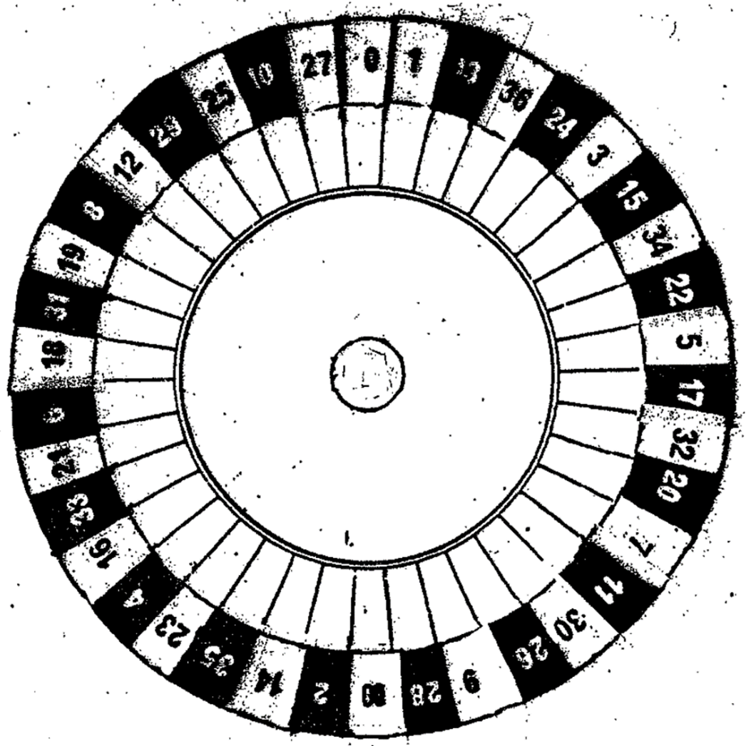
Figure 1. American roulette

American roulette follows a trichotomy rule or a three-way division in which 36 numbers are equally divided into three sets. Then, a double-looping technique is applied; in which numbers in each set are selected methodically. Such looping techniques are common in modern computer pro programming although roulette was invented at a much earlier date. It is known that Pascal invented the first calculating machine in 1642. Although the inventor of roulette is remained anonymous; it is possible that Pascal simultaneously invented the game.

The procedure of making an American roulette is as follows:

Step 1. Two zeroes are placed in the front. 36 numbers are equally divided into three sets as shown in Figure 2.

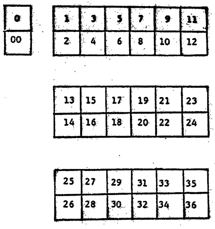
Figure 2. Framework of roulette

Step 2. The numbers in each set are now selected methodically: (a)the tiles of numbers 1 and 2 are taken from the first set, (b)the tiles of numbers 13 and 14 from the second set, (c)and the tiles of numbers 35 and 36 from the far end of the third set, inversely. (d)the tiles of numbers 23 and 24 are taken from the far end of the second set, also inversely. The result is shown in Figure 3. (Note: the shadowing parts also indicate the direction of each move).

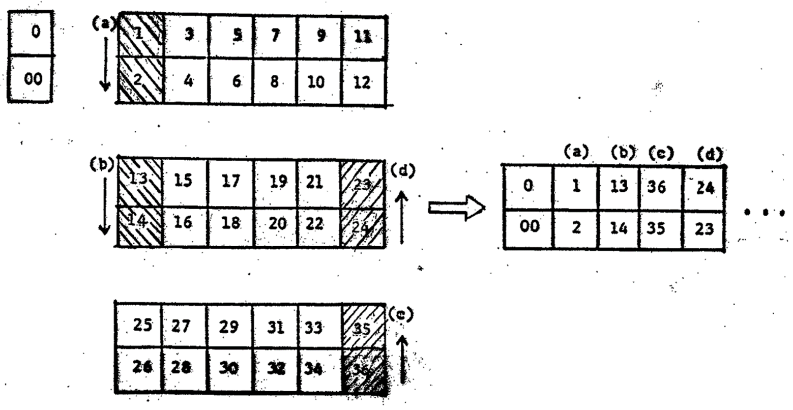
Figure 3. Illustration of steps in making a roulette.

Step 3. The same process is repeated. (a)the tiles of numbers 3 and 4 are taken from the first set, (b)the tiles of numbers 15 and 16 from the second set, (c)and the tiles of numbers 33 and 34 from the far end of the third set, inversely, (d)the tiles of numbers 21 and 22 are taken from the far end of the second set, also inversely.

Step 4. Again, the same process is repeated. (a)the tiles of numbers 5 and 6 are taken from the first set, (b)the tiles of numbers 17 and 18 from the second set, (c)and the tiles of numbers 31 and 32 are taken from the far end of the third set, inversely, (d)the tiles of numbers 19 and 20 are taken from the far end of the second set, also inversely.

Step 5. At this point, all the tiles in the second set have been used up. Consequently, (a)the tiles of numbers 7 and 8 are taken from the first set, (b)the tiles of numbers 11 and 12 from the first set, and (c)the tiles of numbers 29 and 30 from the third set, inversely, (d) the tiles of numbers 25 and 26 are taken from the third set, also inversely.

Step 6. Finally, (a)the tiles of numbers 9 and 10 are taken from the first set. (b)the tiles of numbers 27 and 28 are taken from the third set, but inversely.

All these results, so far, are shown in Figure 4 as follows:

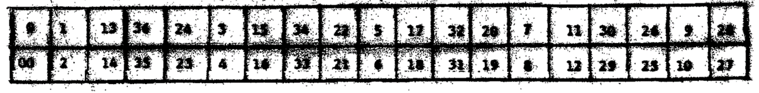
Figure 4. Completed number-arrangement for a roulette

Next, these two rows of numbers are separated and connected from end to end. When expanded into a full circle, it is an American roulette wheel, Now, the odd and even numbers naturally appear in every other two spaces, also it is alternatively in color of red and black in every other single space. Thus, American roulette may not completely reserve the idea of randomness, it does carry the beauty of symmetry to its utmost.

3. The Solution to European Roulette

The diagram of a European roulette is shown here in Figure 5. In this diagram, the number 0 is colored green. Then, starting with number 32, the red and black spaces are colored alternatively.

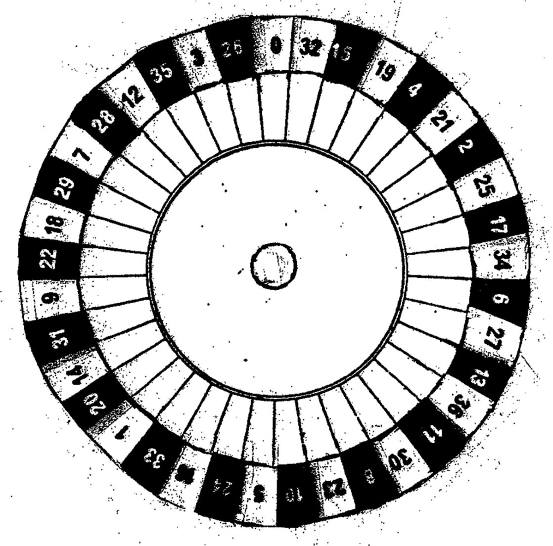
Figure 5. European roulette

The making of European roulette is a little more sophisticated than that of American roulette. It preserves the idea of randomness better, but does not possess the beauty of symmetry. The procedure of making a European roulette, step by step, is as follows:

Step 1. Place the single-zero in the front, the equally divide all other 36 numbers into 4 rows with 9 numbers in each row. The first row includes numbers 1 to 9, the second row includes numbers 10 to 18, the third row includes numbers 19 to 27, and the fourth row includes numbers 28 to 36, We shall randomly select one number from each row. The interesting thing is that the row selection is also random.

In the very first round, we randomly select number 7 from the first row, number 16 from the second row, number 25 from the third row, and number 35 from the fourth row, we call these four numbers our insertion group, since we want to put these numbers aside for the time being, and to be inserted later.

Up to now, the framework for a European roulette looks like Figure 6.

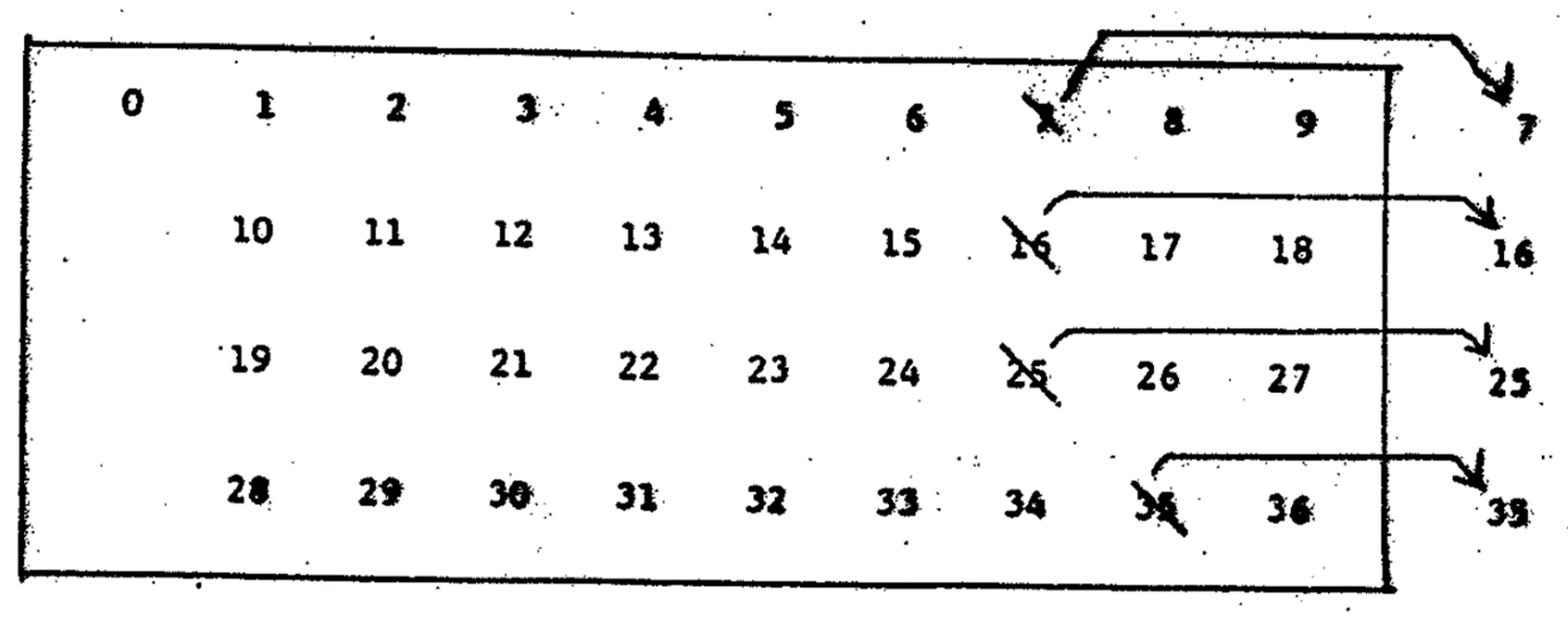
Figure 6. Framework of European Roulette

Step 2. In the second round, (a)take number 32 from the fourth row, (b)take number 15 from the second row, (c)take number 19 from the third row, and (d) take number 4 from the first row, Notice that the row selection continues to be random. These four numbers are our first group. The situation now is shown on the framework is as Figure 7.

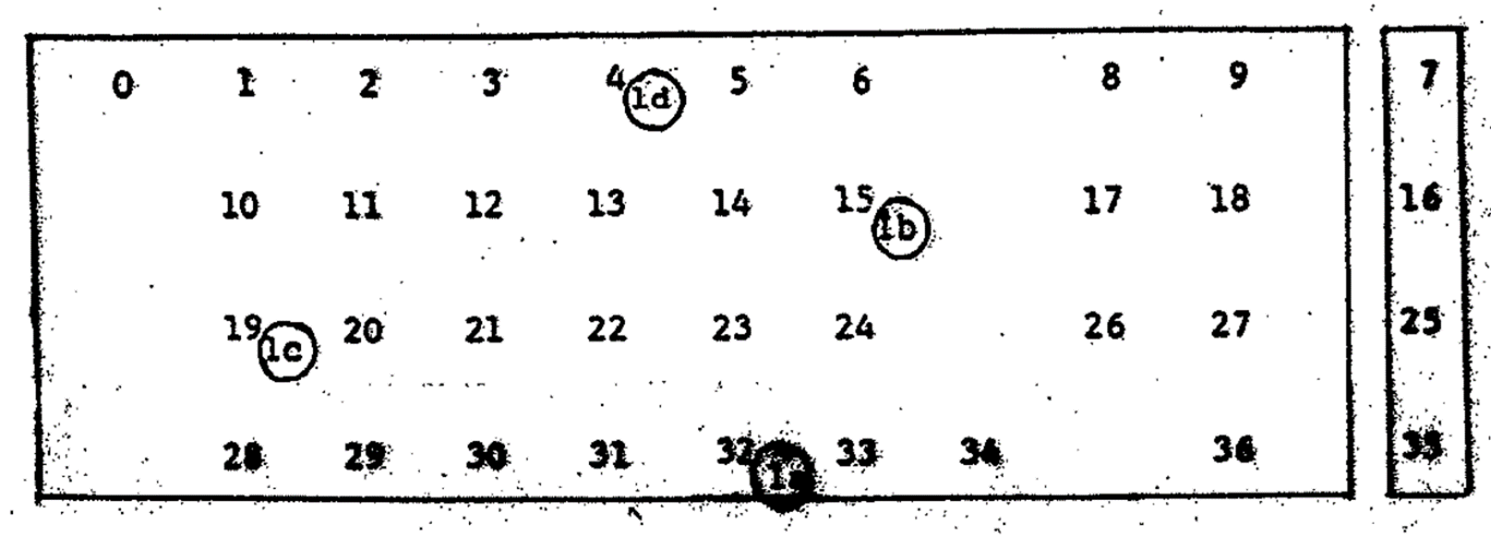
Figure 7. Second step shown on framework of European roulette

Step 3, In the third round, (a)take number 21 from the third row, (b)take numb number 2 from the first row, (c)take number 17 from the second row, and (d)take number 34 from the fourth row. These four numbers are called our second group.

Step 4. In the fourth round, (a)take number 6 from the first row, (b)take number 27 from the third row, (c) take number l3 from the second row, and (d)take number 36 from the fourth row. These four numbers are called our third group.

Step 5. In the fifth round, (a)take number 11 from the second row, (b)take number 30 from the third row, (c)take number 8 from the first row, and (d)take number 23 from the third row. These four numbers are called our fourth group.

Step 6. In the sixth round, (a) take number 10 from the second row, (b)take number 5 from the first row, (c)take number 24 from the third row, and (d)take number 33 from the fourth row. These four numbers are called our fifth group.

Step 7. In the seventh round, (a)take number 1 from the first row,(b)take number 20 from the third row, (c)take number 14 from the second row, and (d)take number 31 from the fourth row. These four numbers are called our sixth group.

Step 8. In the eighth round, (a)take number 9 from the first row,(b)take number 22 from the third row,(c)take number 18 from the second row, and (d)take number 29 from the fourth row. These four numbers are called our seventh group.

Step 9, In the final round, (a)take number 28 from the fourth row,(b)take number 12 from the second row,(c)take number 3 from the first row; and (d)take number 26 from the third roW. These four numbers are called our eighth group.

We have completed our selection process, and the current situation can be shown on the framework as in Figure 8.

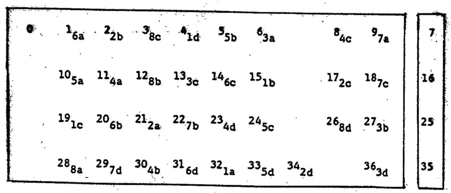
Figure 8. Final stage of number-arrangement on the framework of a European roulette

Step 10. After the completion of selection process, all the groups are in good order. Now we shall expand it into a full circle with the single-zero in the very front. Keep in mind that, up to now, our insertion group is still outside, no action has been taken.

Next, we start our insertion process, we shall insert those four remaining numbers into the circle at random. The current situation of framework is shown in Figure 9.

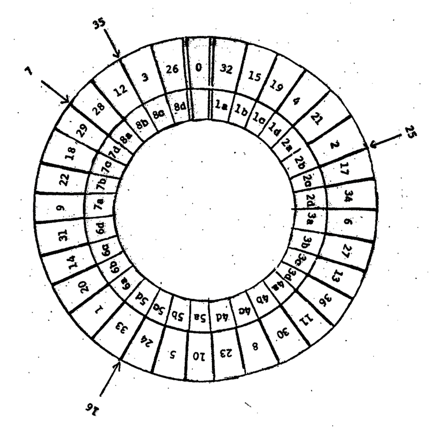
Figure 9. Framework of European roulette before the insertion process

Step 11. This is our final step of making a European roulette. After the completion of insertion process, we shall color the red and black alternatively on each single space. The European roulette, or the French roulette, is completed. Its diagram actually had been shown as our Figure 5 previously.

4. “Red-odd versus Black-even” Differential

We shall discuss an important fact of roulette in this section. It is known that, in a roulette, its red numbers are always equal to its black numbers, and its odd numbers are always equal to its even numbers, they are 18 each. But, it is far from the general thinking that its red-odd numbers are equal to its red-even numbers, and its black-odd numbers are equal to its black-even numbers; they should be 9 each, accordingly. In fact, there are 10 red-odd numbers and 8 red-even numbers, and there are 10 black-even numbers and 8 black-odd numbers. This statement is held true for both American and European roulette wheels. Readers may verify this by checking both American and European roulette layouts which are shown here as figure 10.

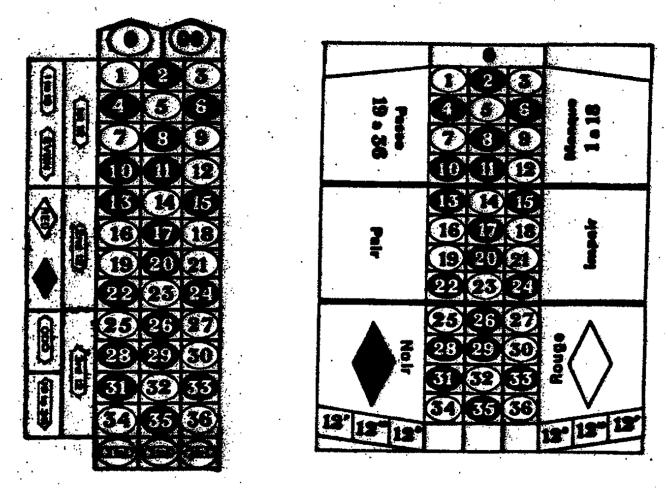
Figure 10. American and European Roulette Layouts

We name this differential as “red-odd versus black-even” for convenience. Literally it should be named as “red-odd versus red-even, and black-Odd versus black-even” differential.

Obviously, this fact shall affect the play. Suppose that a player makes a simple bet on red, black, odd, even, small (which means numbers

1 to 18), or large (which means numbers 19 to 36), We call these simple bets as our normal play. Consequently,

The probability of winning is 18/38 = 0.4737.

The probability of losing is 20/38 = 0.5263 (due to the existence of 2 zeroes).

The difference between the winning and losing probabilities is 0.0526, which also represents the house advantage of having two zeroes since 2/38 = 0.0526.

Suppose that the player now makes a compound bet on red and odd at same time, It follows:

The probability of winning is 10/38 = 0.2632.

The probability of losing is 12/38 = 0.3158.

The probability of ending as draw is 16/38 = 0.4210.

The same probabilities are also true for betting on black and even at the same time. Also the difference between the probabilities of winning and losing is again 0.0526. We consider such a compound bet a less aggressive play while compared with a normal play since it generates a draw case. The chance of being a tie game is 0.4210. In other words, there is about 42% of the time the player will end up as draw.

Next, suppose that the player makes a compound bet on red and even at same time. It follows:

The probability of winning is 8/38 = 0.2105.

The probability of losing is 10/38 = 0.2632.

The probability of ending as draw is 20/38 = 0.5263.

The same probabilities are also true for betting on black and odd at same time. The difference between the probabilities of winning and losing is again 0.0526. We consider such a compound bet a least aggressive play while compared with a normal play. The chance of being a tie game is 0.5263. In other words, there is about 52% of the time the player will end up as draw.

For a European roulette which is the single-zero case, the probabilities can be computed basically the same way. Suppose that a player makes a simple bet on red, black, odd, even, small, or large numbers, or a normal play. It follows:

The probability of winning is 18/37 = 0.4865.

The probability of losing is 19/37 = 0.5135.

The difference between the winning and losing probabilities is 0.0270, which also represents the house advantage due to having single-zero since l/37 = 0.0270.

Suppose that the player now makes a compound bet on red and odd at same time. It follows:

The probability of winning is 10/37 = 0.2703.

The probability of losing is 11/37 = 0.2973.

The probability of ending as draw is 16/37 = 0.4324.

The same probabilities are also true for betting on black and even at same time. The difference between the probabilities of winning and losing is again 0.0270. We consider such a compound bet a less aggressive play while compared with a normal play since it generates a draw case. The chance of being a tie game is 0.4324. In other words, there is about 43% of the time, the player will end up as draw.

Next, suppose that the player makes a compound bet red and even at same time. It follows:

The probability of winning is 8/37 = 0.2162.

The probability of losing is 9/37 = 0.2432.

The probability of ending as draw is 20/37 = 0.5405.

The same probabilities are also true for betting on black and odd at same time. The difference between the probabilities of winning and losing is again 0.0279. We consider such a compound bet a least aggressive play while compared with a normal play. The chance of being a tie game is 0.6405. In other words, there is about 54% of the time the player will end up as draw.

The basic idea of such a differential can be shown geometrically in a diagram. See Figure 11.

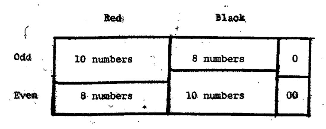
Figure 11. Diagram of “Bed-odd versus Black-even” Differential

The question follows is that is it possible or not to eliminate this differential. With the current 36-number scheme (0 and 00 uncounted for), it is not possible. Only with a 48-number scheme, it can be done. Simply add one more set of 12 numbers (from 37 to 48), then apply the same looping technique to Section 2 previously discussed, we shall not repeat it here. In other words, we shall have 12 each for red-odd, red-even, black odd, and black-even numbers. Of course, the odds, payoffs, and layouts all have to be adjusted accordingly. This new modified roulette may not be practically useful, since it further reduces the winning chance on a single-number bet which is already hard enough under current scheme. However, it is the only alternative or possible trade-off.

5. A “Success-region” Method

In this method, we view the roulette as a spinning wheel experiment. The wheel is to be scaled from 0.00 to 1.00 uniformly. For each space, or equal interval, the probability for the spin to stop is the same. This approach has been firstly mentioned by Fraser. * The theory behind such an experiment is uniform distribution. For an uniform probability distribution, its probability density function is

and its distribution function is , or

As we apply it to roulette, we shall let a-value = 0, and b-value = 38. Since we have 38 space, or equal interval, on our wheel, and the probability for the spinner stopping on each space is 1/38 = 0.0263.

There is a good reason to use uniform distribution here. After the non-randomness of number-arrangement had been proved, we may consider the numbers on a roulette wheel is no longer a set of random or discrete numbers, but a sequence of natural numbers. Therefore, the success-region technique means to select an adequate segment of the sequence.

Mathematically, it can be stated as follows.

Let A_i be the probability of choosing ith number for our player, then P(A_i) = 0.0263, with i = 1,…, 38, and

Then, a player will choose his success-region as

and his failure region will be

The key words in this method is segment or partial sequence. In other words, we are choosing several numbers in an entire sequence to cover the winning number as possible; through the use of uniform distribution.

Besides, in the process of making an American roulette, we found that for a three-way division, the probabilities for each region are not equal, two regions have higher probabilities than the other one. Cross reference with Figure 2 in Section 2 will be helpful. This finding also can support our theory. This particular situation can be illustrated in Figure 11.

Figure 11. Illustration of “Success-region”(Same area but with unequal probabilities).

6. Random walk or Markovian model

In this section we shall discuss the classical gambler’s ruin problem, which presents a typical a random walk or Markovian model. It can be formulated as follows: A gambler has k units capital, and his opponent has (a-k) units capital. Therefore, the total capital in the game is a, since k + (a – k) = a. The probability of his winning is p, and the probability of his losing is q. Also p + q= 1. For each win, our gambler receives one unit of capital from his opponent, and for each loss, he pays one unit of capital to his opponent. Apparently, our gambler is taking a random walk along the capital axis. If he reaches the left end, which means his ruin. If he reaches the right end, which means his success (gaining all the capital).

Let us only concentrate on the probability of his ruin: Given all the a, k, p, and q values, and let q_k indicates the probability of the gambler’s eventual ruin; all we need to do is to solve a first order difference equation:

q_k = p*q_k+1+ q*q_k-1

with boundary condition q₀ = 1, and q_a = 0.

Its solution had been offered by many statisticians and mathematicians as follows:

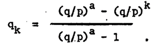
An algebraic solution also provided by Kemeny, Snell and Thompson. By substituting p/q = r, r<l, then q/p = 1/r. The answer is:¹

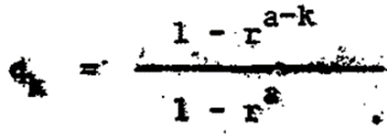
The discussion of “classical gambler’s ruin” problem is necessary here since it applies to all games of chance. My point is that since the number-arrangement on roulette wheels had been proved not random, “red-odd versus black-even” differential has been revealed, and it is also found that for some areas the probabilities are not equal. These facts indicate that roulette is not flawless, it is not a perfect game of chance. These facts could offset some of house advantages. In some cases, one play can have advantage over the other, for example, playing red and odd against playing red and even, etc. In other words, after non-randomness has been proved, roulette may not belong to random walk or Markovian models, therefore, the “classical gambler’s ruin” may not apply to the case of roulette.

7. Conclusions

Roulette is an interesting and also intrigue game. It has perplexed people for quite some time. It is about time for roulette to be solved completely. In this paper I had revealed some of its secrets, if not all. I have a few conclusions.

One of my main purpose is to make my colleagues aware that not to use roulette to be an example of randomness in writing statistical texts. This is a common error, some have done so. I have no difficulty to provide you some book titles at any time, or you can find by yourself on your bookshelf. Even Von Neumann and Morgenstern might have overlooked on this in their classical work.2

Since I am a statistician, not gambler; the statistical proof is my top priority, winning comes second. This does not mean that statistician cannot win. In this paper, I had clearly solved the structural or hardware-part problem of a roulette. To guarantee the win, one needs to do some more homework which means the software-part. I believed that both classical statistics and Bayesian approach can produce winning programs. In other words, there may be only one solution for hardware, but there are more than one solutions for software. Another analogy is that just like building economic model, the structural equation is given, but still needs to fill in the coefficients.

In this paper, I had mentioned computer, but I did not use computer. Anyone had fundamental statistical training can tell that all I had applied is statistical reasoning. It is quite a manual or human job, not a computer job. Roulette-is a typical problem for statisticians, not for mathematicians or computer programmers; for operational researcher, may be. Of course, I shall not underestimate the power of computer, it will be very useful in next step – to Write winning program as I mentioned -in last paragraph.

There is a conclusion on the theoretical aspect. After the non-randomness had been proved, and “red-odd versus black-even” differential had been revealed, roulette may be no longer belongs to a family of random walk or Markovian models. Therefore, the “classical gambler’s ruin” may not apply to the case of roulette. It further leads to the conclusion that roulette is no longer to be a game of chance. Of course, more research is needed along this direction.

___________________________________________________

Note: I had developed my two basic solutions rather early. In 1982, there was an article in September issue of JASA, mentioned that roulette is a statistical problem. By-then, land-based gambling was overwhelmingly prohibited, even now, it is limited to riverboats or Indian reservations. I just copyrighted my solutions at same year. When I worked on the enlarged version-of this paper, I found that if one goes deep on roulette strategies, it will become a trade book or “How to” book, it gradually loses statistical meaning. I repeat one more time that I am statistician, not gambler, and not intend to write a winning guide for gamblers. On the other hand, one should not use heavy mathematical tools to solve an elementary problem. These two factors affected the format of this paper, I considered it as a piece of academic work. After all, roulette is just a puzzle for statisticians. This leads to a common sense conclusion that good statisticians can always make good gamers or gamblers, but not vice versa. This also could be extended as: If that is the case, “A.S.A. versus casinos”, then I will place my bet on the former without question.

The views expressed in this paper are those of the author and no official endorsement by the MDOT is intended or should be inferred.

I would like to thank Professor J. Stuart Hunter (our President) for approval of this topic, so I can present this paper in the Section of Statistics and Sports/Games. Due to the dual nature of the topic; it is fifty-percent statistics and fifty-percent gambling with rather more emphasis on the latter, I believed that the gamblers should also be informed too, so I had presented a paper of similar version (i.e. with two basic solutions) at a Conference of Gambling and Risk-taking sponsored by the Gambling Research Group of University of Nevada-Reno in August, 1987. It was well-received. Of course, gamblers are more interested in winning rather than studying the random walk or Markovian models, but they also can appreciate the discussion of “classical gamblers’ ruin” and “gambler’s fallacy”, etc. A more broad-based discussion on the theoretical aspect of this topic is included in later sections (sections 5, 6, and 7) in this paper.

*See D,A.S. Fraser,”Statistics, An Introduction”, New Yorkr Wiley, 2nd.ed. 1960, pp,65-67.

1. See Kemeny, J.G., J.L. Snell, and G.L. Thompson, “Introduction to Finite Mathematics”, 1966. pp. 210-212.

2. Von Neumann, J., and O. Morgenstern, “Theory of Games and Economic Behavior”, Princeton University Press, 1947. p. 87.

REFERENCES

PROBABILITY AND STATISTICS

Bailey, N.T.J., “The Elements of Stochastic Process”, New York: Wiley, 1964.

Bownlee, K.A., “Statistical Theory and Methodology in Engineering and Sciences”, New York: Wiley, 2nd.ed., 1960.

Draper, N.R., and Lawrence, W.E., “Probability”, Chicago; Markham Co., 1970.

Feller, W., “An Introduction to Probability Theory and Its Application”, Volume 1, New York: Wiley, 2nd.ed., 1960.

Fraser, D.A.S., “Statistics – An Introduction”, New York: Wiley, 2nd.ed., 1960.

Kemeny, J.G., and J.L. Snell, and G.L. Thompson, “Introduction to Finite Mathematics”, Englewood Cliff: Prentice Hall., 1966.

Von Neumann, J., and O. Morgenstern, “Theory of Games and Economic Behavior”, Princeton, N.J.: Princeton University Press, 1947.

COMBINATORICS

Riordan, J., “An Introduction to Combinatorial Analysis”, New York: Wiley, 1958.

CRYPTOGRAPHY

Konheim, A.G., “Cryptography, A Primer”, New York: Wiley, 1981.

Sinkov, A., “Elementary Cryptanalysis”, New York: Random House, 1968.

GAMBLING AND GAMES

Frey, R.L., “According to Hoyle”, Greenwich, Conn.: Fawcett, 1970.(paper back).

Silberstang, J., “The Winner’s Guide to Casino Gambling”, New York: New American Library, 1980.

A Solution To Roulette